Because precision GPS positioning requires differencing of carrier phase, we choose to tightly constrain (effectively fix) one site in the network (REYK) at its International Terrestrial Reference Frame 1997 (ITRF97) [Boucher et al. (1999)] coordinates for each week. The coordinates of REYK are referred to epoch 1997.0 and are projected to its present ITRF97 position using the ITRF97 velocities. Thus the daily coordinate results can be considered to be in the ITRF97 reference frame. After the data have been downloaded from the receivers, they are converted to RINEX (Receiver INdependent EXchange) format [Gurtner (1994)] using UNAVCO's teqc software [Estey and Meertens (1999)]. When data from all stations have been collected, usually between 5 and 6 am GMT, preliminary results (coordinates) are automatically calculated using predicted satellite orbits from the Center of Orbit Determination in Europe (CODE). The results are readily used to update images on the ISGPS web pages that are used for monitoring activity in the crust. Later the data are reprocessed using CODE final orbits [Hugentobler et al. (2001]. In both phases of processing we use the rapid pole information BULLET_A.ERP [McCarthy (1992)], [McCarthy (1996)]. The quality of CODE predicted and final orbits differs by a factor 4 [Hugentobler et al. (2001] and is reflected in poorer quality of the results obtained using the predicted orbits.
The daily coordinate results are transformed to a local east-north-up coordinate system and
the displacement since a fixed epoch calculated relative to REYK
to build up the time series. The associated daily coordinate error is taken as the square root of the diagonal
elements in the daily solution covariance matrix after transforming it to a local east-north-up
coordinate system. We refer to this error as the "formal coordinate error". The off-diagonal
elements in the full covariance matrix, representing the correlation of the coordinate results between
coordinate compononents and stations, are generally not zero. The off-diagonal elements in
the full covariance matrix are not taken into account in this study.
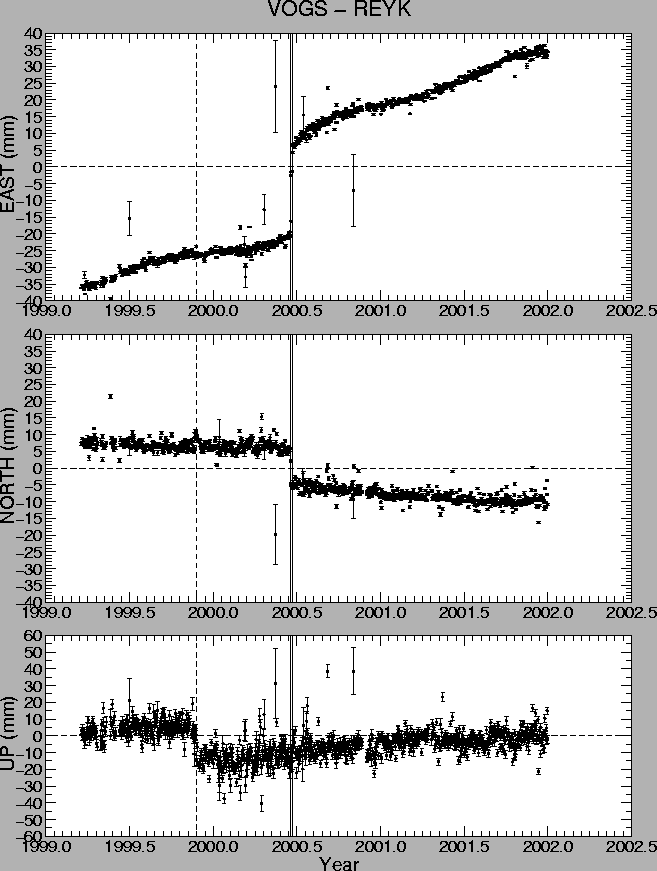 |
Figure 5 shows an example of the resulting time series. The figure shows the diplacements of VOGS relative to REYK as a function of time. The plate movements appear as gradual displacement towards east and south in Figure 5. As a first approximation we can assume that the plate velocities are constant. The errorbars in Figure 5 are the formal coordinate errors. The errors are not the true coordinate errors, as they are underestimated by the Bernese processing software [Hugentobler et al. (2001)] and need to be rescaled to obtain a more rigorous estimate of the coordinate errors. Incorrect coordinate errors lead to wrong error estimates for offsets in the time series, e.g. due to the June 2000 SISZ earthquakes and radome installation. Section 3.1 describes how the formal coordinate errors are rescaled.
There are a few outliers in the time series that need to be removed before the data are used for further interpretation. Outliers can substantially bias plate velocities derived from the time series (Section 4). The outliers can be removed by visual inspection, but that is not feasible since it is time consuming and it is hard to keep consistency for all the stations. Section 3.2 describes how the outliers are detected and removed.