Detection of outliers

Outlier detection is an important part when post processing of the data since outliers can easily bias estimations of plate velocities and obscure other signals in the time series. Outliers can be caused e.g. by short or bad data files at stations. High ionospheric activity can also corrupt the data, but for many outliers it is impossible to say why they lie far from neighbouring data points. From Figure 5 we can see there are two types of outliers: Type 1 - data points with abnormally large errors and Type 2 - data points with normal errors but lie abnormally far from its neighbouring data points. Consequently the outlier removal is performed in two steps, removing outliers of Type 1 in the first step and outliers of Type 2 in the second step. When an outlier is detected in one coordinate component, the other 2 components for the same day and station are deleted from the time series.

We define Type 1 outliers as data points with error larger than 3 times the median error (Table 4) for each component at each station. The median is a much more robust estimator than the mean in the presence of outliers. Before outlier detection, the median and mean of the formal coordinate errors for the east component of VOGS were 0.240 and 0.310 respectively. After the outlier detection the corresponding values were 0.238 and 0.259, emphasizing that the median is a more appropriate estimator of the average than the mean when outliers are present.

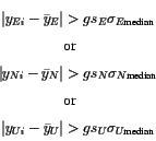
Outliers of Type 2 are harder to deal with. We must define what we mean by the expression "abnormally far from neighbouring data" and care must be taken not to remove data that actually are far from its neighbouring data due to offsets in the time series (Figure 5). To detect outliers of Type 2 we first remove from the time series known jumps due to earthquakes and radome installation. The time series, for each component of each station, are then split into time intervals including e.g. 50 data points each (discussed later in this section) and the median value of the coordinates is calculated for each time interval. Again we choose to use the median instead of the mean because it is a more robust estimator. If a coordinate value lies more than four times the scaled median coordinate error (already calculated in step 1) from the median coordinate value of each time interval, then the point is considered an outlier of Type 2. Stated a bit more mathematically the criteria for a point to be considered an outlier of Type 2 is

$$\begin{split} \vert y_{E i} - \bar{y}_{E} \vert & > g s_{E} ... ...} \vert & > g s_{U} \sigma_{U \textrm{median}} \\ \end{split}$$ (4)

where y_i is the coordinate value, $\bar{y}$ is the median coordinate value within each time interval, g is a gain factor that controls how strict the outlier conditions are, $\sigma_{\textrm{median}}$ is the median of the formal coordinate error (from step 1), and s_E, s_N and s_U are the scaling factors (see Section 3.1). The labels E, N and U refer to the coordinate components.

For the outlier detection scale factors s_E = s_N = 4.0and s_U = 2.5 were used. The gain factor g controls how far from its neighbours a point is allowed to be without being considered an outlier. The conditions become stricter as g is smaller. Values for g ranging from 1 to 10 were tested. Values below 2 were way too stringent and many points in the data series were removed (16% of data points removed for station VOGS for g = 2). Values above g = 5 proved to be too large and many obvious outliers were not detected (2% of data points removed for station VOGS for g = 8). A value of g = 4.0 (4% of data points removed for station VOGS) was finally used for the outlier detection.

The length of the time interval used in the outlier detection was varied between 20 and 200 data points. If the time interval is too long, then valid data points are considered outliers because the data are not detrended and higher order signals in the time series start to interfere at time intervals of 100 to 200 days. A too short time interval follows the data values too closely and leaves many outliers undetected. A time window of 50 data points was used for the final outlier detection.

The method does not account for gaps in the data. Since gaps in the data are usually much shorter than 50 days, this is not considered important. It was only at station HLID that this caused problems and a few valid data points were removed from the time series near large gaps (see Figure 9). These data points were added to the time series again afterwards. A small deformation signal observed at SOHO in relation to the Hekla 2000 eruption was removed from the time series by the outlier detection scheme. This caused some valid data points to be considered as outliers and they were added to the time series afterwards.

The outlier detection has a significant effect on the scaling factors obtained (see Section 3.1) because outliers can greatly bias the estimation of WSTD (equation 2). Vice versa the scaling factors affect the outlier detection through equation 4. In practice the outlier detection and scaling factor estimation were made in an iterative manner -- starting with a scaling factor of 3 to find an appropriate value of g, which is then used in the scaling factor estimation (outliers are removed prior to the estimation) and the new scaling factor used in the outlier detection etc.